Microblogging is becoming more and more ubiquitous among today’s generation. In fact, interactions on some type of online platform or service such as Facebook, Twitter or Google leave traces of data that show a record of behavior or actions. As Davidowitz put it in his book Everybody Lies: “The everyday act of typing a word or phrase into a compact, rectangular white box leaves a small trace of truth that, when multiplied by millions, eventually reveals profound realities.” To statisticians, this quote faintly reminds of the many statistical ideas that could be put to the test.
An emerging role of online platforms has been in the political context. As such, our research interest would be to predict political outcomes with a preferred dataset that is in line with our hypothesis and allows us to scientifically control for many variables.
Hypothesis: We could use sentiments on social media to predict public opinions as a proxy for political outcomes.
The scope of the preferred dataset(s) that we are looking into include observations
- whose geolocations match those of the political outcomes of interest.
- represent the voter base. And;
- are longitudinal.
To that end, we gathered the following dataset from Kaggle:
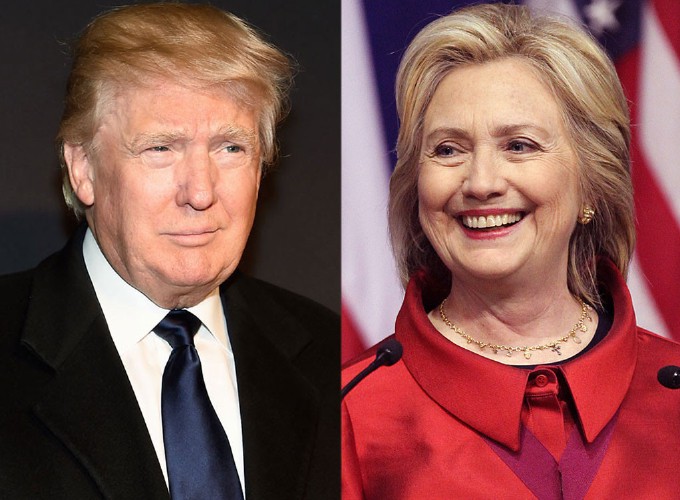
Hillary Clinton and Donald Trump Tweets
| Features | Description |
|---|---|
| handle | Twitter handle name |
| text | Tweets |
| is_retweet | Whether the tweet was retweeted |
| original_author | Original author |
| time | Timestamp |
| in_reply_to_screen_name | - |
| in_reply_to_status_id | - |
| in_reply_to_user_id | - |
| is_quote_status | Whether the tweet was quoted |
| lang | Twitter’s guess at language |
| retweet_count | Retweet count |
| favorite_count | Favorite count |
| longitude | Longitude |
| latitude | Latitude |
| place_id | Place id |
| place_full_name | Place full name |
| place_name | Place name |
| place_type | Place type |
| place_country_code | Country code |
| place_country | Country |
| place_contained_within | Place contained within |
| place_attributes | Place attributes |
| place_bounding_box | Place bounding box |
| source_url | Tweet source url |
| truncated | Whether it is truncated |
| entities | a JSON object |
| extended_entities | Another JSON object |
The dimensions of the dataset:
## [1] 7468 3First five observations of both candidates:
@HillaryClinton:
##                                                                                                                                          text
## 1         Thank you @_VicenteFdez. You're right—"su voz es su voto." So grateful to have your support. #JuntosSePuede https://t.co/j9v2K84AV1
## 2                   No matter where you live you can make sure you're registered to vote at https://t.co/tTgeqxNqYm.… https://t.co/tWlu8DiGIg
## 3 RT @azcentral: The Arizona Republic ed board has endorsed @HillaryClinton. See why: https://t.co/FqStTwkesL via @azcopinions #elections2016
## 4          20 years after Donald bullied a beauty pageant winner for her weight the real "problem" is...still Donald. https://t.co/ZmqYWuN9px
## 5                   The question in this election: Who can put the plans into action that will make your life better? https://t.co/XreEY9OicG
##                  time         handle
## 1 09-28-2016 02:36:13 HillaryClinton
## 2 09-28-2016 02:10:42 HillaryClinton
## 3 09-28-2016 01:19:46 HillaryClinton
## 4 09-28-2016 01:13:08 HillaryClinton
## 5 09-28-2016 00:22:34 HillaryClinton@realDonaldTrump:
##                                                                                                                                             text
## 4191 My supporters are the best! $18 million from hard-working people who KNOW what we can be again! Shatter the record: https://t.co/8ZHGyOth0f
## 4192   Unbelievable evening in Melbourne Florida w/ 15000 supporters- and an additional 12000 who could not get in. Tha… https://t.co/VU5wh2zXBU
## 4193                      Join me for a 3pm rally - tomorrow at the Mid-America Center in Council Bluffs Iowa! Tickets:… https://t.co/dfzsbICiXc
## 4194     Once again we will have a government of by and for the people. Join the MOVEMENT today! https://t.co/lWjYDbPHav https://t.co/uYwJrtZkAe
## 4195 RT @GOP: On National #VoterRegistrationDay make sure you're registered to vote so we can #MakeAmericaGreatAgain https://t.co/GKcaLkx8C8 ht…
##                     time          handle
## 4191 09-28-2016 02:17:06 realDonaldTrump
## 4192 09-28-2016 01:03:03 realDonaldTrump
## 4193 09-27-2016 22:13:24 realDonaldTrump
## 4194 09-27-2016 21:08:22 realDonaldTrump
## 4195 09-27-2016 20:31:14 realDonaldTrump
According to Google Trends, the keywords most searched on Google during the 2016 election are “Abortion”, “Immigration”, “Race Issues”, “Economy”, “Affordable Care Act”, “ISIS”, “Climate Change”, “National Debt”, “Gun Control” and “Voting System.” Using gtrendsR, we randomly picked five of those keywords and queried its search hits by setting geo = "US" to prevent bias.
trend1 = gtrends(c("immigration", "abortion", "economy", "gun control", "terrorism"), geo = "US", time = "2016-01-01 2016-12-31")

plot(trend1)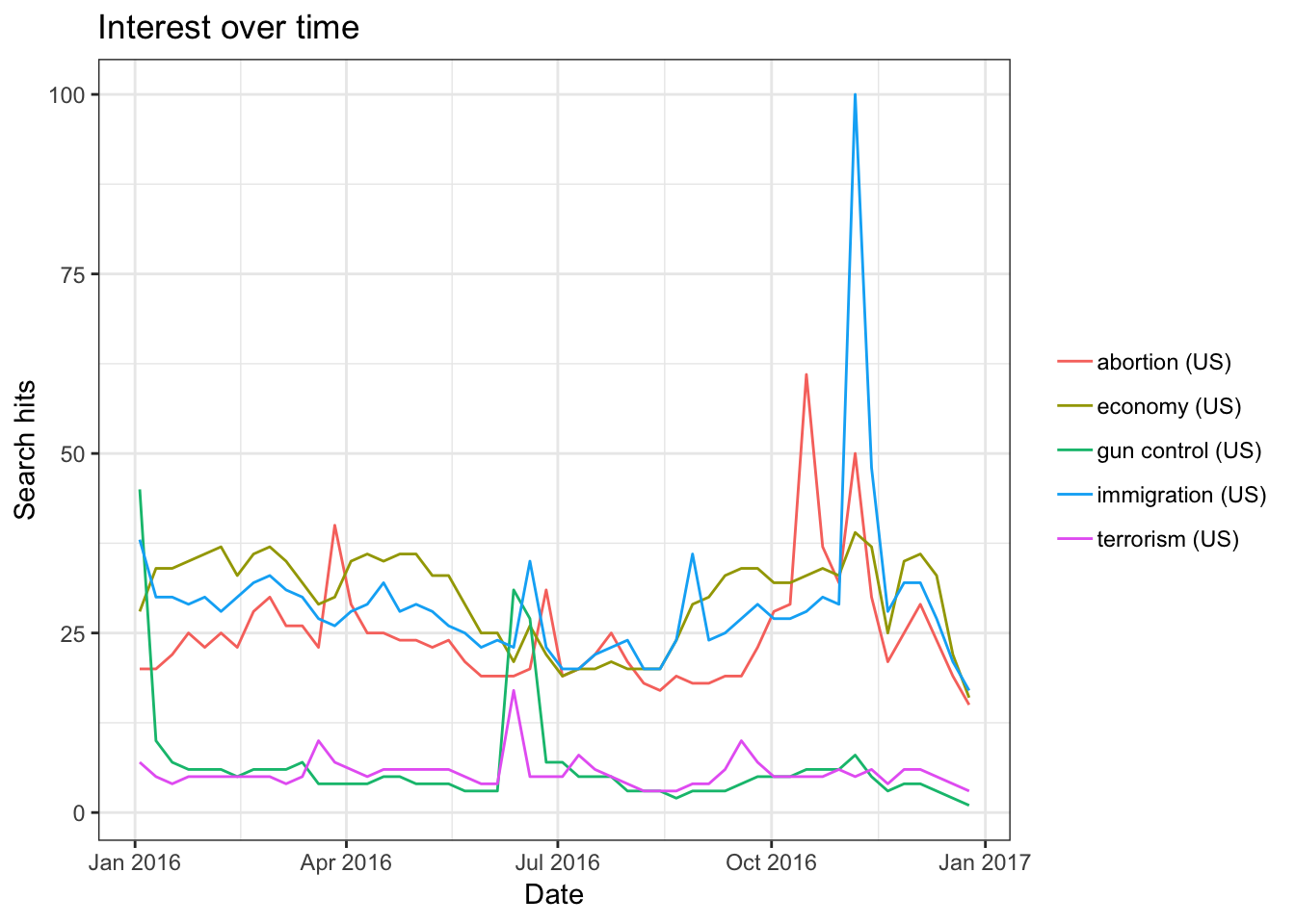
Lo and behold, the trends do not differ much when we queried for Trump and Hillary.
trend2 = gtrends(c("hillary", "trump"), geo = "US", time = "2016-01-01 2016-12-31")

plot(trend2)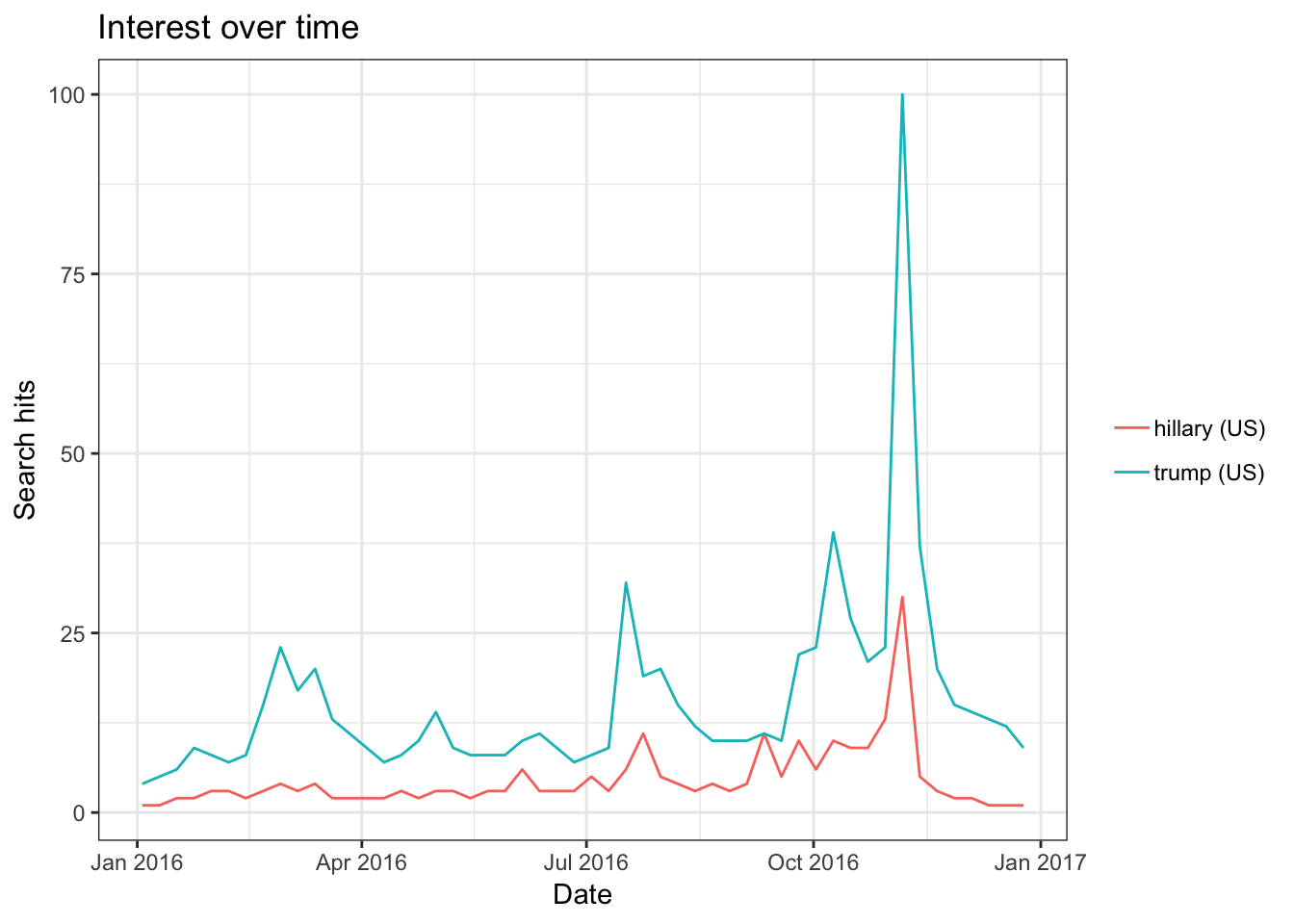
The trends show the relative popularity of the search query adjusted by the total number searches and time period. We see that these trends look more similar around mid-campaign.
Another popular measure of public opinions are by using polls. To that end, we queried HuffPost Pollster, a poll that aggregates every poll that claims to represent the population using pollstR.
We obtained the following charts using the slug 2016-general-election-trump-vs-clinton with pollstR:
## Warning: The `printer` argument is deprecated as of rlang 0.3.0.
## This warning is displayed once per session.
trend.plot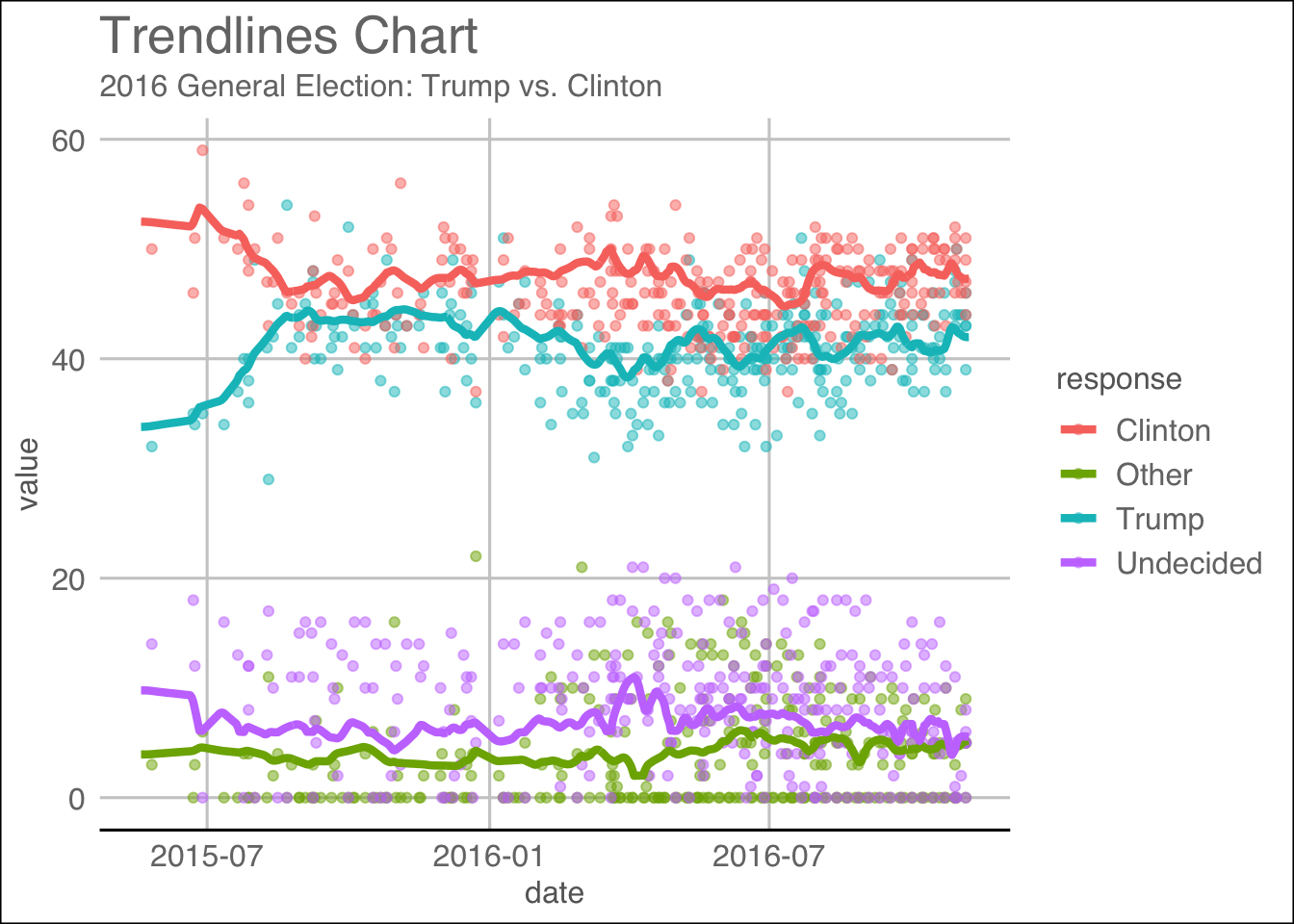
We hypothesize that these trends are invoked by the use of sentiments from both political candidates during their campaigns either through speech or social media. Using the trends as the labels and the sentiments as the features, we could attempt to build a model to find out their relationship.
Literature Review
If I have seen further it is by standing on the shoulders of Giants.
— Isaac Newton
Indeed, the Google search engine is seen as this black box that confounds from the feeblest to the strongest of men. Only until recent years that it is seen as a treasure trove to people who analyze big data. Seth Stephen-Davidowitz, a former data scientist at Google, addressed in his book Everybody Lies: Big Data, New Data and What the Internet Can Tell Us that
… there’s something very comforting about that little white box that people feel very comfortable telling things that they may not tell anybody else about: Their sexual interests, their health problems, their insecurities. And using this anonymous aggregate data we can learn a lot more about people than we’ve really ever known.
This reveals an implicit truth: that these data probably understand people more than they do about themselves. Thus, on account to this, many have studied google search queries in hopes to uncover this social behavior. As the Japanese say there are three faces of self: one you show it to the world, the second you show to your close friends, and the third you don’t show it to anyone. For whatever reason, people seem to comfortable with telling everything to the white little box on a daily basis.
Another popular metric to “quantify” this social behavior is by using polls that are collected by surveyors. These polls are taken and studied insofar as they represent the population, as written by Huffpost Pollster. The survey questions on the polls are designed so much so that that they are unbiased so the survey takers would be able to answer them impartially. However, over the recent years, there have been counless debates against the credibility of the polls.
As evident during the 2016 US election, Hillary Clinton led the popular votes by a huge margin and that the polls predicted that she would be the one to take oath of office at the beginning of the next term. However, the contrary happened and that our reliance on predictive analytics on reams of data had outstripped the understanding of its limitations: that they are tools of probabilistic estimate, but still quite useful. A paper written by Kassraie, Modirshanechi & Aghajan (2017) attempted to do just that. The authors collected tweets from the public during the election and aggregated their sentiments so that they could be used to perform some predictive evaluation onto weekly election polls. They fitted a linear model by first choosing an uncorrelated set of features that would make the regression’s dimensions perpendicular. The poll ratings are then used as the response. The results are shown on these graphs:
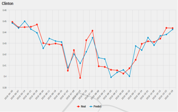
Figure 1: Predicting online election polls with sentiment data for Clinton.
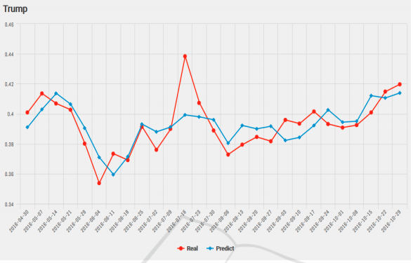
Figure 2: Predicting online election polls with sentiment data for Trump.
As far as prediction goes, using sentiments on social media to predict election polls can be seen as a viable choice given the above result. Of the two predictions, the model on Clinton achieved a mean error of 0.50 % and that on Trump achieved a mean error of 1.08 %.
As alluded previously, prediction using polls as a means of predicting political outcomes has received many criticisms. One of the criticisms allegedly claimed that polls failed to capture the caprice of voters. For example, a Trump loyalist may vote in favor of the opposing party on the online polls but might have behaved otherwise when they cast ballot. For this reason and more, we will attempt to predict social behavior by using as Google Trends with our Twitter dataset.
Approach/ Design/ Analysis
Sentiment Analysis
Before performing any ML algorithm on our dataset, let us take a peek into it by performing some sentiment analysis. After “cleaning” the tweets by removing the links, special characters, and stop words, we could obtain the following plots:
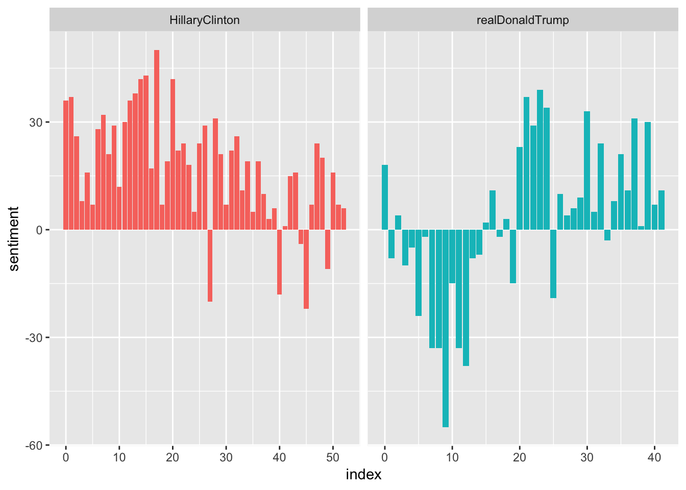
This plot shows the number of sentiments used by each candidate over time. Note that this sentiment analysis is based on the frequency at which the word appear on the Twitter dataset. From the plot, we could generally see that one of the candidate’s sentiments are more geared towards the negative, while the other seems remain stable around the positive side fof the rhetoric.
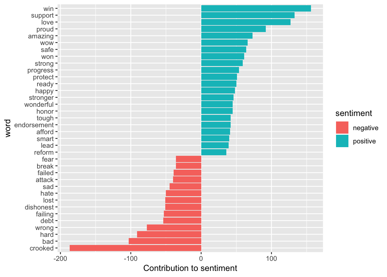
Now, from this plot, we can see the words that are contributing to the sentiments from the most positive to the most negative. Here, we chose the words that appear at least 35 times for better interpretation. Knowing this information is useful in designing and validating our hypothesis.
Prediction
Define a popularity vector \(\mathbf{P}\) as
\[\mathbf{P} = \frac{|\{w_i : w_i \in W\} |_t}{|W|_t} \in \{[0, 1]\}_{t=1}^n\]
, which is approximately how the Google Trend’s search hits are defined after adjusting for time. We want to estimate \(\mathbf{\hat{P}}\) using the sentiments to predict social behavior.
To that end, we would like to design a document-term matrix by keeping only the sentiments and and then fit several models to estimate the Google Trends.
1) Cleaning the data
We are mostly interested in the tweets of the dataset and their timestamps, hence we would like to clean them so that we will only get the sentiments to obtain the document-term matrix. We will use the tm package to achieve that.
The following code is used to obtain the document-term matrix:
# Obtaining a corpus object

corpus = as.character(tweets_mutated[, "tweets"]) %>%
  removeURL %>%
  removeSpecial %>%
  stemWord %>%
  VectorSource %>%
  VCorpus

# Transforming the corpus

cleaned_corpus = tm_map(corpus, tolower) %>%
  tm_map(PlainTextDocument) %>%
  tm_map(removePunctuation) %>%
  tm_map(removeNumbers) %>%
  tm_map(removeWords, stopwords("english")) %>%
  tm_map(stripWhitespace)

# Obtaining the Document Term Matrix

DTM = DocumentTermMatrix(cleaned_corpus) %>%
  removeSparseTerms(0.99) %>%
  as.matrix

# Merging the data

res_H = cbind.data.frame(DTM, "hits" = tweets_mutated$hillary_hits/100 )
res_T = cbind.data.frame(DTM, "hits" = tweets_mutated$trump_hits/100 )
The idea is to pipeline the tweets from the dataset through a process of transformations. An initial glimpse of the data reveals that the some of the tweets have links and special characters (such as emojis) that needed to be removed, hence we created the functions removeURL and removeSpecial to do just that. Furthermore, we recognized that, depending on the context, some words mean the same thing, hence we had to “stem” the words so that they will return to their original word. A function called hunspell_stem() from the hunspell package allowed us to do just that (and more efficiently than a similar from the tm package). The function is included in the functional stemWord so that the tweets that go through it will return the word in its root form.
Suppose a vector of characters:
[1] "loving" "love" "loved" "lovely"
Depending on the context, we would want a vector that would be expressed as following:
[1] "love" "love" "loved" "love"
This process is important so that the document term matrix can pick up on the frequency at which the sentiments appear since it usually returns a matrix that is sparse and that that would be problematic when interpreting the results. Furthermore, we let the tweets ran through some more functions like tolower,removePunctuation, removeNumbers, removeWords (to remove English stopwords) and stripWhiteSpace to obtain tweets of only sentiments.
Note that before we had to go through this process, we had to concatenate the strings by each day to match with the number of hits we have since we have too have them by day. This is in line with our hypothesis that the search hits are not only affected by the sentiments invoked by one candidate individually, but rather collectively.
After transforming the tweets, we transformed them into a document-term matrix and remove sparse terms.
The dimension of our document-term matrix is:
dim(DTM)## [1] 268 226And now, we are ready to do our analysis.
2) Logistic Regression
With the dataset, we attempt to fit a logistic regression since our relative popularity (i.e. search hits) is designed to be bounded from 0 to 1 and signify proportions. First, we will crudely fit the response with all of the features. Once we do that, we will get the following results:
Hillary’s search hits logistic diagnostic:
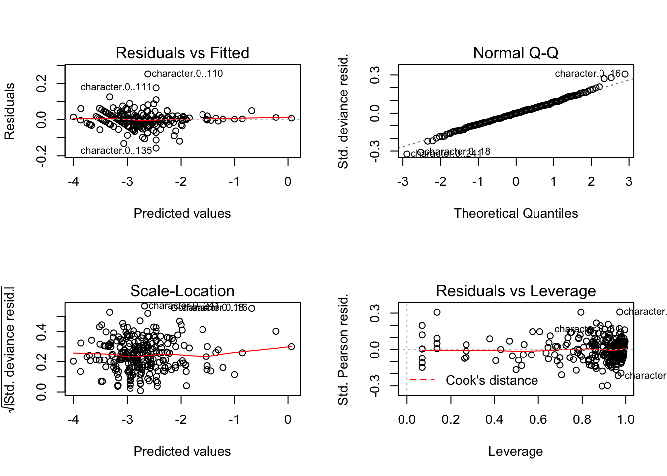
Trump’s search hits logistic diagnostic:
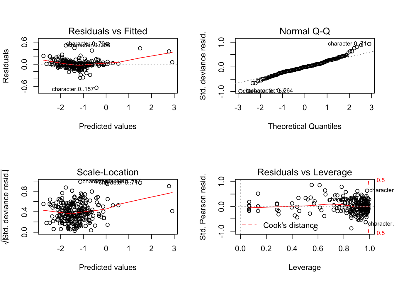
If we look at the diagnostic, we see that none of the assumptions for inference are violated, so we could easily perform the usual hypothesis testings. From the plots, we see that we almost perfectly fit the trends with the given design matrix. For both of the models, we obtain the following Mean Squared Error (MSE):
# MSE for Hillary's model (adjusted for scale)
mse(logit_H$fitted.values,res_H$hits)*100^2
## [1] 1.043019# MSE for Trump's model (adjusted for scale)
mse(logit_T$fitted.values,res_T$hits)*100^2## [1] 22.39258However, if we care about parsimony, we may wish to perform some variable selection with AIC since AIC generally works well with prediction and that it penalizes much less. To that end, we will use the stepAIC() function:
# Number of features used

## On Hillary's GTrends
length(AIC.glm_H$coefficients) - 1
## [1] 226## On Trump's GTrends
length(AIC.glm_T$coefficients) - 1 ## [1] 226We see that none of the variables were penalized, hence the MSEs for both models remain the same. This variable selection method does work that well because the directional variable selection has a one-way solution path thus it may not exhaust all possible subset selection.
3) LASSO vs Ridge Regressions
We may also be interested in doing a penalized linear regressions to find out which variables matter more in the estimate. Two of the most common penalized regressions are the LASSO and Ridge regressions, with the former penalizes the coefficients more. Since our design matrix is a document-term matrix, some terms may not be that useful, hence using the penalized regressions can help us ignore those variables. We attempt to tune the penalty for LASSO first:
# LASSO fit for Hillary
cvH.fit=cv.glmnet(as.matrix(res_H[,1:227]),as.matrix(res_H$hits),type.measure="mse")
plot(cvH.fit)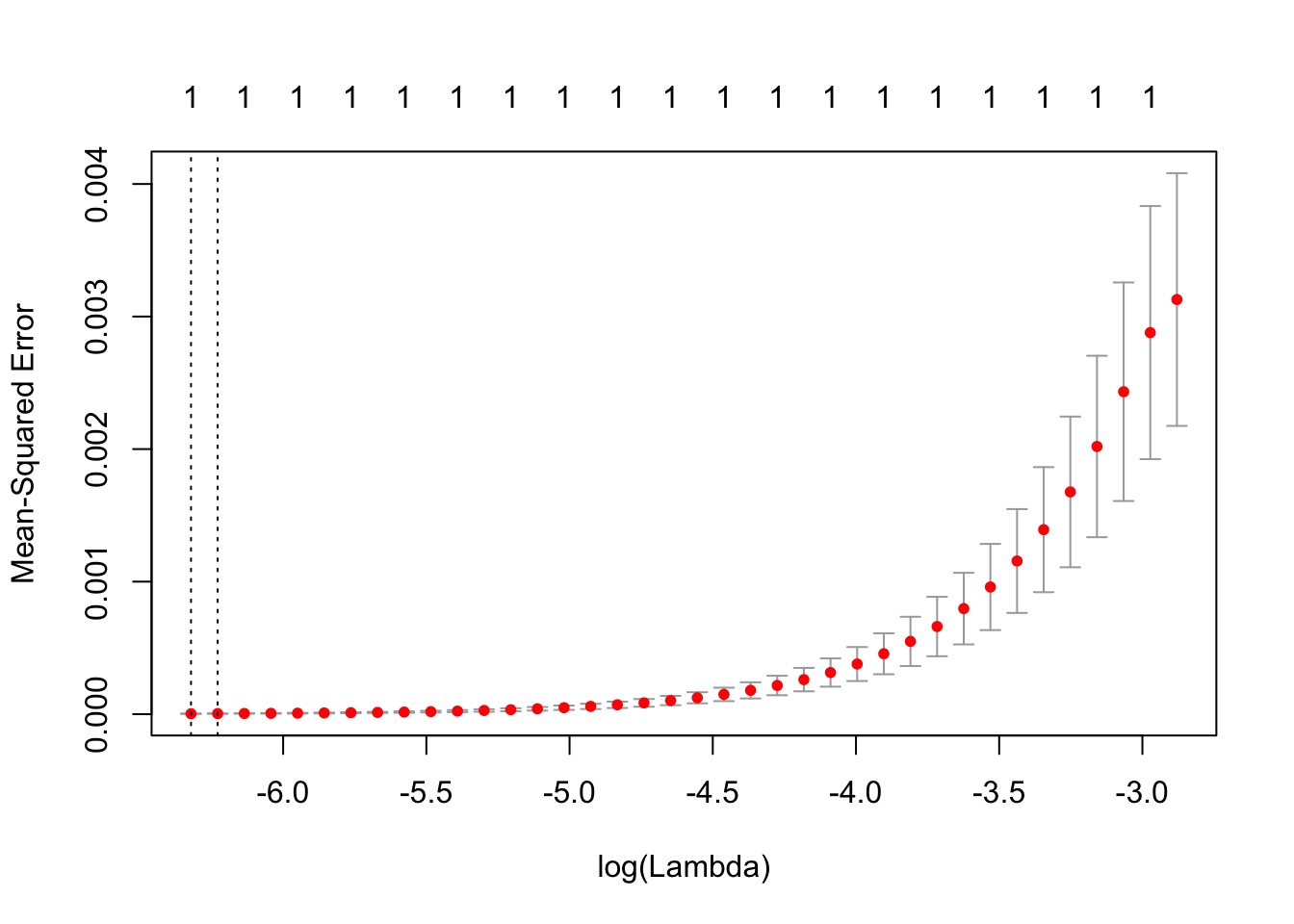
# LASSO fit for Trump
cvT.fit=cv.glmnet(as.matrix(res_T[,1:227]),as.matrix(res_T$hits),type.measure="mse")
plot(cvT.fit)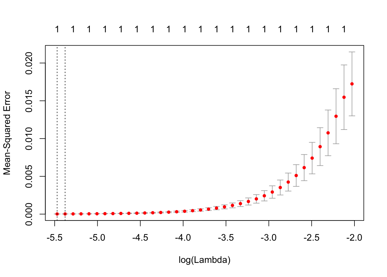
# The tuning parameters

## For Hillary
cvH.fit$lambda.1se
## [1] 0.001972102## For Trump
cvT.fit$lambda.1se## [1] 0.0046166The parameters chosen here are the ones that minimize the MSE, hence we will be using them as the parameter to fit our models.
## MSE for Hillary's LASSO model (adjusted for scale)
mse(yhat111,res_H$hits)*100^2
## [1] 0.03889185## MSE for Trump's LASSO model (adjusted for scale)
mse(yhat222,res_T$hits)*100^2## [1] 0.21313We see that the MSE for both of the plots seem to fit perfectly, which is a concern since we have a sparse matrix. Due to this, performing a gradient descent will not be meaningful.
Futhermore, we may now wish to perform a Ridge regression.
# Define a sequence of lambdas
l = seq(0, 1000, by = 0.01)

# Fitting the models with lambdas
ridge.H = lm.ridge(hits~., res_H, lambda = l)
ridge.T = lm.ridge(hits~., res_T, lambda = l)

# Plotting GCV against lambdas

plot(ridge.H$lambda, ridge.H$GCV, col = "darkorange" ,type = "l", ylab = "GCV", xlab = "lambda", main = "GCV against lambdas for Hillary's Ridge Regression")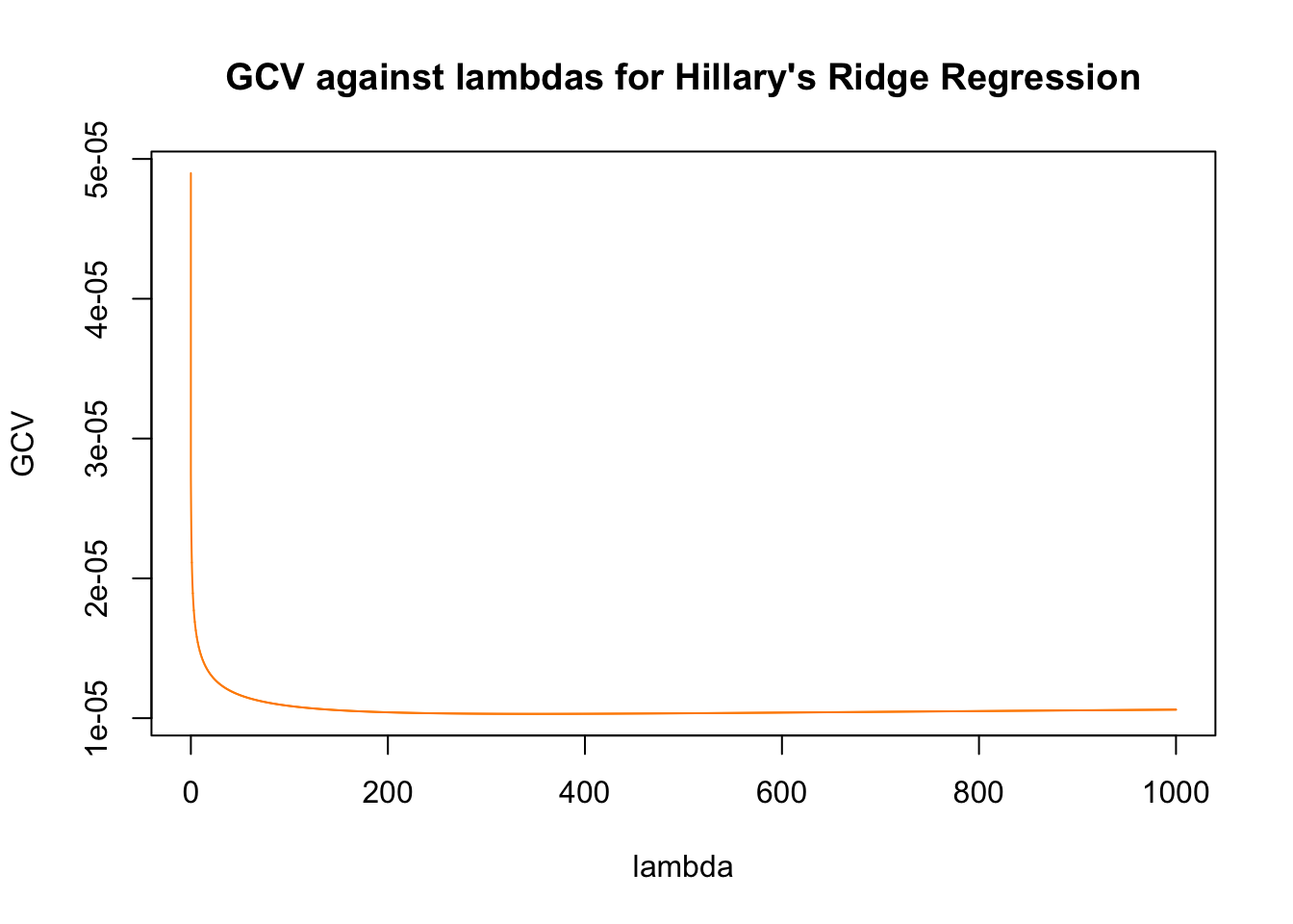
plot(ridge.T$lambda, ridge.T$GCV, col = "darkorange" ,type = "l", ylab = "GCV", xlab = "lambda", main = "GCV against lambdas for Trump's Ridge Regression")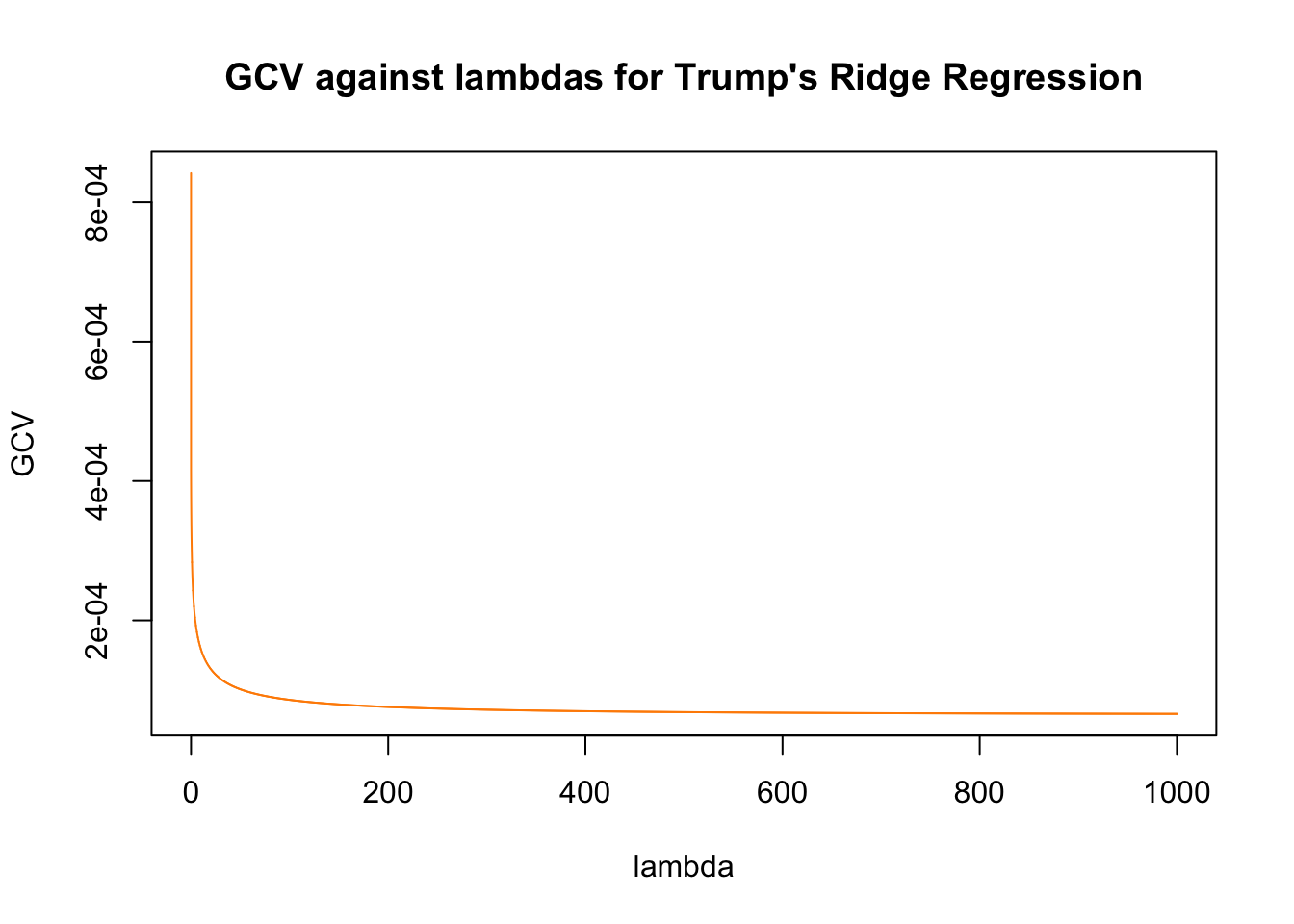
Similar to LASSO, the Ridge regression has the same tuning parameter for penalty, which we will tune differently than LASSO by using the GCV metric. After obtaining the minimum GCV that corresponds with the lambdas, we will then use that lambda to fit our models.
The following are the MSE’s for both models:
## MSE for Hillary's Ridge model (adjusted for scale)
mse(y.pred.H,res_H$hits)*100^2
## [1] 14.93831## MSE for Trump's Ridge model (adjusted for scale)
mse(y.pred.T, res_T$hits)*100^2## [1] 130.2933We see that Ridge regressions perform badly for Trump’s Google Trends hits relative to that of Hillary. We say that this might be due to the sharp peaks that the Trump’s hits may have, or that maybe it is due to the dataset being collected since Trump’s tweets are fewer than Hillary’s.
4) Random Forest
With Random forest we first try the default version, and realize that by simply doing randomForest() and setting up the ntree we still have a pretty bad model. Therefore we start tunning the parameters of mtry and ‘nodesize’:
We can see that Clinton ’s optimal mtry is 80 and optimal nodesize is 32. Trump’s optimal mtry is 77 and its optimal nodesize is 37.
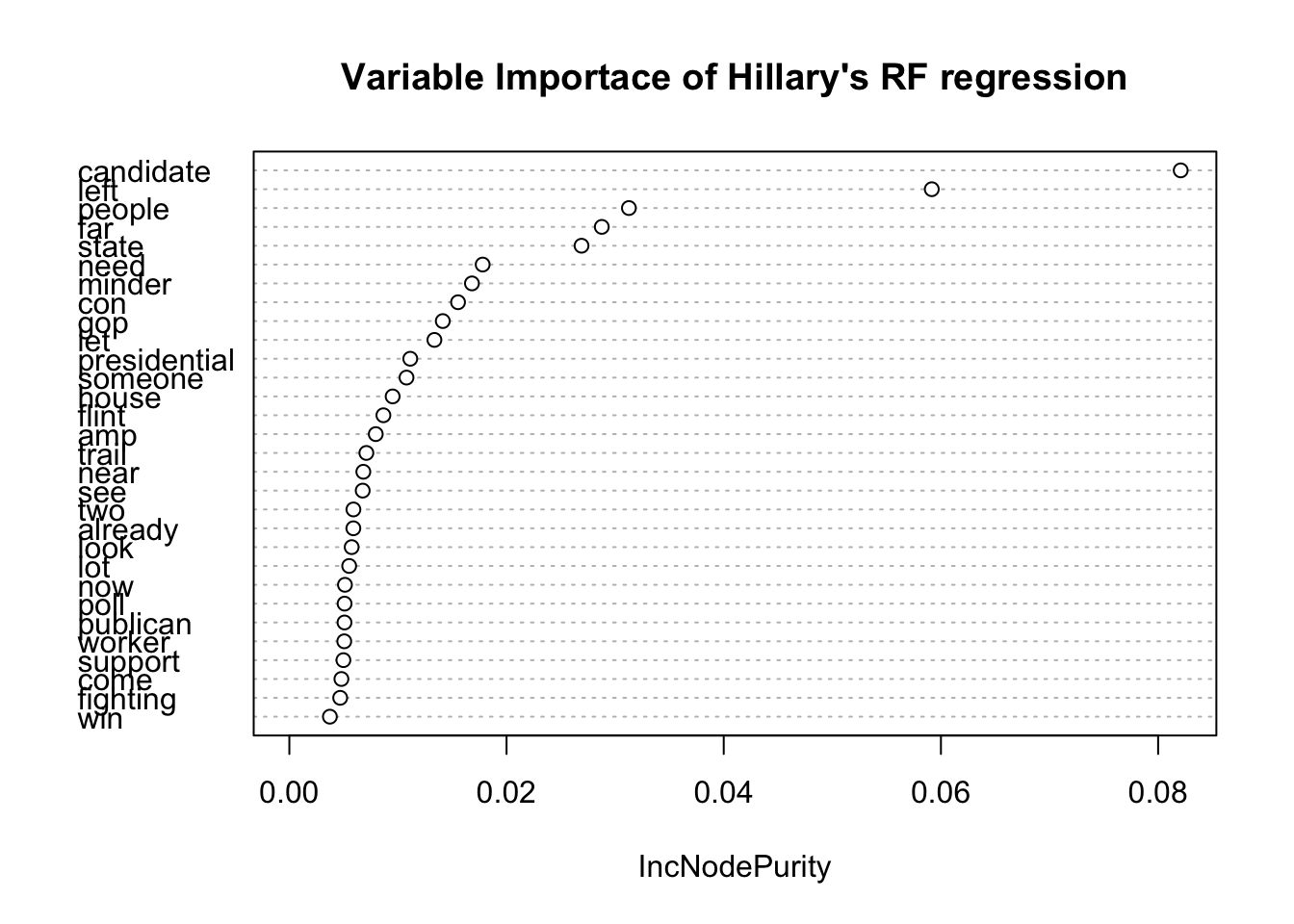
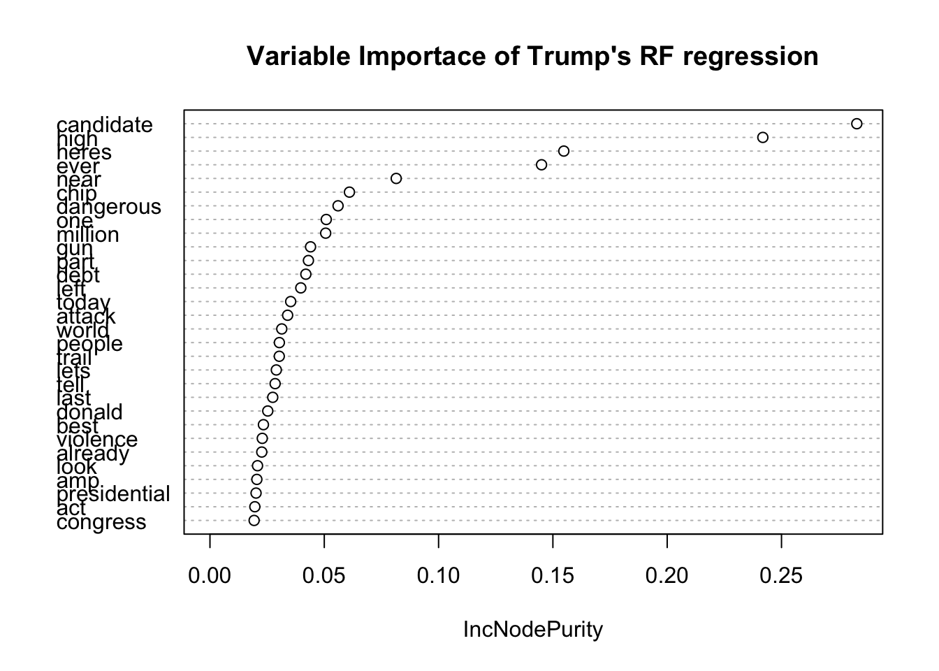
From the variable importance plots of both models, the term candidates seem to show up the most in both.
The result of the Mean Squared Errors are listed as follows:
## MSE for Hillary's RF model (adjusted for scale)
mse(rf.H$predicted, res_H$hits)*100^2
## [1] 35.92742## MSE for Trump's RF model (adjusted for scale)
mse(rf.T$predicted, res_T$hits)*100^2## [1] 224.50755) Feature Selection
We could attempt to find the features that greatly affect the prediction. However, since we have features of only factor variables, computing the distance matrices may be a problem. As such, we could use the FactoMineR package to solve this problem since it would allow us to compute the principal components for mixed variables
fact = res_H[,1:226] %>% lapply(as.factor) %>% do.call(cbind, .)
res.pca=PCA(fact[,1:226])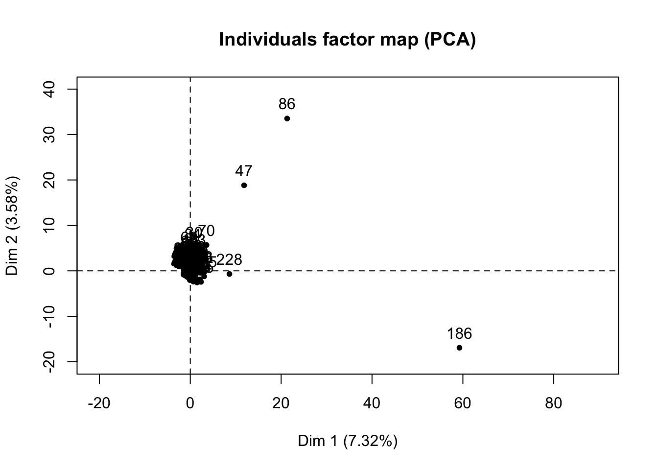
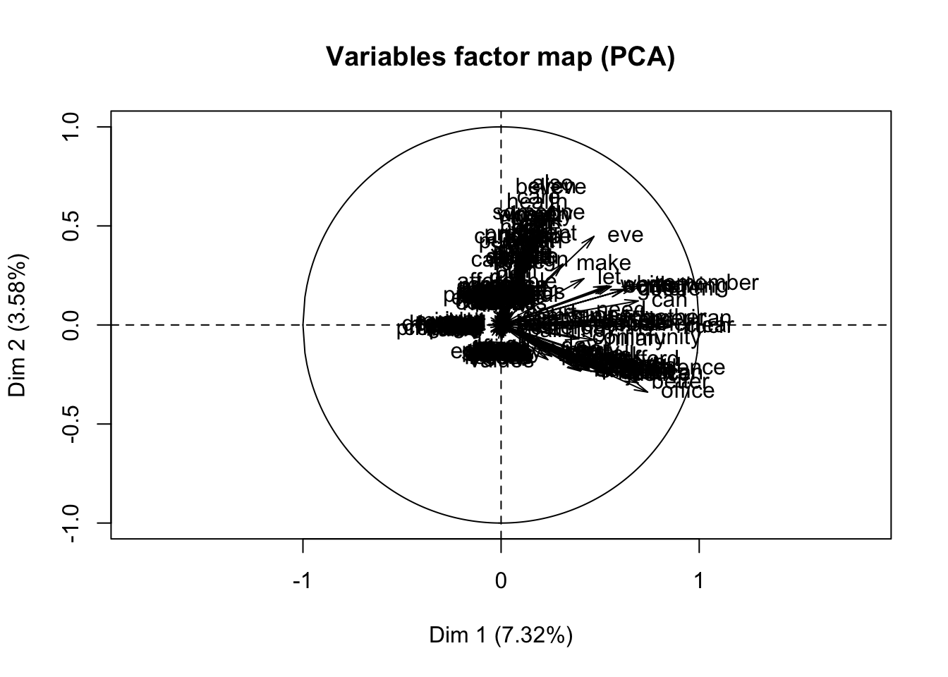
We see that doing a feature selection by PCA from each of the plots since they did not contribute too much to the explanations of the variance for both dimensions. Therefore, we say that using PCA on a document-term matrix may not work that well since our variables are not continuous.
Discussion
From the results, we see that the outcome of our prediction vary a lot based on the characteristics of the methods we applied and how certain methods are impacted by the data sets.
For the logistic model, by applying AIC for variable selection, we see that none of the variables were removed. This method may not work that well since the solution path may be one-way only, not exhaustive. Another method that we could have done is to use the best subset selection, which does an exhaustive search on all features to find the best subset of features that would fit the model best.
For the penalized regression models, we see that we encounter a problem with overfitting for the LASSO regression model. This may be due to the document term matrix being sparse, so LASSO had to force its ranks on all the covariates. Although we fit an almost perfect linear model with substantially low MSE, this may not be desirable if we take into account parsimony and the bias-variance tradeoff. For the Ridge regression, we found out that the model on Trump’s search hits did not work that well. If we examine the comparison plots closely, we found that the predicted values did not fit well when the trend had some sharp peaks. Furthermore, this may be due to the fact that Trump’s tweets are fewer than Hillary’s, which may have caused the fitted model to work better using Hillary’s search hits than Trump’s.
Using the method of Random Forest, we found that the models did not work that well, even after the we tune for mtry around p/3 and various nodesize. The variable importance also here used IncNodePurity, which may be the default for sparse document term matrix. We also realized that the randomForest() did not list the coefficients for our model, which may also be caused by the model matrix being sparse.
To summarize the methods, we computed the MSEs for each method to compare and contrast:
| Method | Trump | Hillary |
|---|---|---|
| Logistic | 22.43 | 1.05 |
| LASSO | 0.21 | 0.04 |
| Ridge | 130.35 | 15.09 |
| Random Forest | 227.79 | 36.75 |
We see that among the fitted models, the LASSO regression works the best in terms of Mean Squared Errors, while Random Forest performed the worst even after tuning the parameters mtry and nodesize. To present a visual result, we produced the following plots:
H.comparison.plot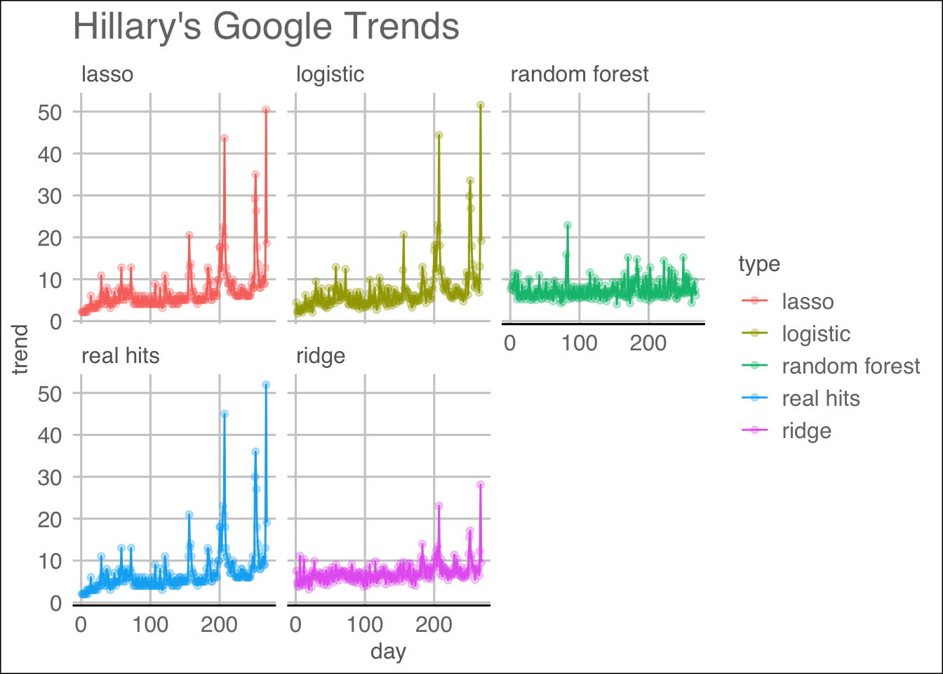
T.comparison.plot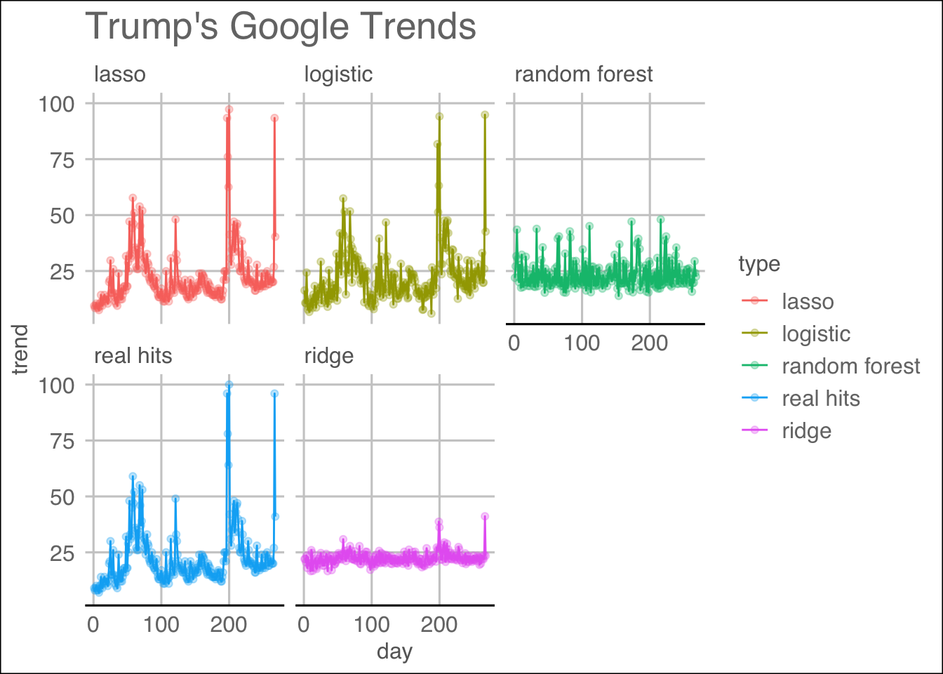
We can see from the visualization which methods follow the patterns well.
Finally, for the feature selection, we used the PCA method to find the features that would explain the variation the most. Given that we have columns of almost binary values, PCA would not work that well since it works best for continous variables. As can be seen from the PCA variance plot, only 7.4% of variation is explained by the terms in the document-term matrix. Another method that could have been done is by using Non-Negative Matrix Factorization (NMF), which may work well on a document-term matrix whose sentiments express themselves well in terms of frequencies at each document.
Conclusion
In conclusion, we can able to say that the sentiments on social media can predict public opinions as a proxy for political outcomes. Our potential pitfalls might be that the number of characters are pretty small for the data set by looking at nchar(), resulting in fewer sentiments for our analysis. If we are doing similar analysis in the future, we might choose data set with greater density for both candidates of the prediction and perform classification to the tweets into any class we are interested in if we have more time.
Reference
Kassraie, Modirshanechi & Aghajan. (2017). “Election Vote Share Prediction using a Sentiment-based Fusion of Twitter Data with Google Trends and Online Polls.” Scite Press, http://www.scitepress.org/Papers/2017/64843/64843.pdf
Stephens-Davidowitz, Seth. (2017). “Everybody Lies: Big Data, New Data, and What the Internet Can Tell Us About Who We Really Are.” The B&N Sci-Fi and Fantasy Blog, Barnes & Noble Reads, https://www.barnesandnoble.com/w/everybody-lies-seth-stephens-davidowitz/1125687298